Finite Volume Method Use

Requirements

Set up acousticDE following the instructions in the installation section of the READme file.
Download and install SketchUp from SketchUp website or use the free web-based platform;
Download and install g-mesh from G-msh website;
Install the MeshKit extension of SketchUp from the extension warehouse.

Usage & files

To use the software, the following files are to be used:

PrepareInputsFVM.py: to create the json file with the inputs of the room;
CreateMeshFVM.py: to create the volumetric mesh using Gmsh software;
FVM.py: it contains the main function run_fvm_sim to run the full simulation and calculate the acoustics parameters in the room.

The main software works with the following associated functions:

FVMfunctions.py includes all the main functions that are used in the full simulation;
FunctionRT.py calculates the reverberation time of the room in question;
FunctionClarity.py calculates the clarity \(C_{80}\) of the room in question based on Barron’s revised theory formula;
FunctionDefinition.py calculates the definition \(D_{50}\) of the room in question based on Barron’s revised theory formula;
FunctionCentreTime.py calculates the centre time \(T_s\) of the room in question based on Barron’s revised theory formula.

Inputs

Geometry & Mesh

The geometry for this method is defined within SketchUp. In order to create a volumetric mesh of the room, the following steps need to be followed in SketchUp:

Create the 3D geometry of the room to simulate in SketchUp, setting the units of the geometry in meters;
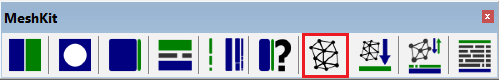
In the MeshKit extension banner in SketchUp software, set the active mesher to gmsh by clicking on the “edit configuration button”
Include the Gmsh Path of the gmsh.exe and select gmsh as the active mesher;
Group the overal geometry (surfaces and edges) bounding the internal air volume by selecting everything, right-clicking and clicking “Make Group”;
Select the Group and click “Set selected as an smesh region and define properties” 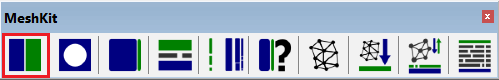in MeshKit;
In the “Region Options: gmsh” menu, keep all the default option but change only the name of the region by writing, for example, “RoomVolume” and click “ok”;
Open the group by double clicking on the object;
Select one or multiple surfaces you want to assign a boundary property;
Click “Add tetgen boundary to selected” 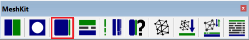in MeshKit;
Under “Refine”, change the refinement to 1;
Under “Name”: change the name to “materialname”, e.g., “carpet” and click “ok”;
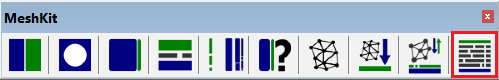
After finishing defining all the boundaries, select the group and click “export to generate mesh” in MeshKit;
Select Format = “gmsh” and Units = “m” and click “ok”;
Keep the default options apart from “pointSizes” which should change to True, click “ok” and save the .geo file with the name of your choice;

The .geo file has been created. This needs to be converted into a .msh file, to get the full volumetric mesh. Using the Download CreateMeshFVM.py script, please input the following variables:

name_of_geo_file: the name of the geo file you want to simulate (e.g. 3x3x3.geo);
name_of_gmsh_file: the name of the mesh file you want this python file to generate (e.g. 3x3x3.msh); and
length_of_mesh: The mesh length value describes the size of the spatial resolution of the mesh in the space and is vital to discretize correctly the space and achieve precise and converged results. Through various trials, it has been established that a mesh length of 1 meter is generally adequate. However, for computations involving complex geometries or small rooms, a smaller length of mesh (0.5 meter or lower) is recommended. The mesh length choice is contingent upon user preferences for details in parameters values, room dimensions but mostly dependent on the mean free path of the room. In fact, the length of mesh would need to be equal or smaller than the mean free path of the room.

name_of_geo_file = '3x3x3.geo'
name_of_gmsh_file = "3x3x3.msh"
length_of_mesh = 1

This script creates the volumetric mesh using Gmsh software. The method is suitable for any type of geometry.

General inputs

The general inputs needs to be set by using the script Download PrepareInputsFVM.py

Please download the script and define the following inputs:

input_data = {
    "coord_source": [1.5, 1.5, 1.5], #source coordinates x,y,z
    "coord_rec": [2.0, 1.5, 1.5], #rec coordinates x,y,z
    "fc_low": 125, #lowest frequency
    "fc_high": 2000, #highest frequency
    "num_octave": 1, # 1 or 3 depending on how many octave you want
    "dt": 1/20000, #time discretization
    "m_atm": 0, #air absorption coefficient [1/m]
    "th": 3, #int(input("Enter type Absortion conditions (option 1,2,3):")) # options Sabine (th=1), Eyring (th=2) and modified by Xiang (th=3)
    "tcalc": "decay" #Choose "decay" if the objective is to calculate the energy decay of the room with all its energetic parameters; Choose "stationarysource" if the aim is to understand the behaviour of a room subject to a stationary source
}

file_path = os.path.join(script_dir, '3x3x3.msh') # Full path to the file

Sound source

The sound sources for this method are defined within the PrepareInputsFVM.py python script. The model allows for the insertion of only one source position per calculation. The sound source is defined as an omnidirectional source. The users can input the position in the room in the variable coord_source in meters in the x,y,z directions.

Receiver

The receivers for this method are defined within the PrepareInputsFVM.py python script. The model allows for the insertion of only one acoustics receiver position per calculation. These are defined as point omnidirectional receivers. The users will input the position of the receiver in the room in the variable coord_rec in meters in the x,y,z directions.

Frequency range

The frequency range for this method is defined within the PrepareInputsFVM.py python script. The frequency resolution should be included as inputs variables fc_low and fc_high; these should be the center frequency of a band. The maximum number of frequencies is set in octave bands and can be choosen by the user. Normally, fc_low is set to 125 Hz and fc_high is set to 2000 Hz. The octave setting must be defined: set to 1 for one-octave bands or 3 for third-octave bands.

Time discretization dt

The time discretization for this method is defined within the FVM.py python script. The time discretization will need to be chosen appropriately. According the Navarro 2012, to get good converged results, the time discretization \(\Delta t\) will need to be defined depending on the length of mesh chosen. To make sure that the predictions converge to a fixed value with a very low error, the following empirical criterion will need to apply.

\[10^{-8} = \Delta t^2 \Delta v^{-2}\]

where \(\Delta v\) is the mesh length chosen. The time discretization is defined in seconds.

Air absorption

The air absorption for this method is defined within the PrepareInputsFVM.py python script. The absorption of air will need to be entered. The air absorption is defined as m_atm and in 1/meters and it is only one value for all the frequency bands.

Absorption Term

In the diffusion equation model, three different absorption term conditions can be used. More info about these terms are shown in the software theory documentation of the FVM. The user can choose the preferred one. The options are Option 1 for the Sabine absorption term, Option 2 for Eyring absorption term and Option 3 for the Modified absorption term. These are absorption factors for the boundary conditions.

Type of calculation

The type of calculation for this method is defined within the PrepareInputsFVM.py python script. The source is defined as an interrupted noise source. The duration for which the source remains on before getting switched off is predefined depending on the theoretical calculated Sabine reverberation time of the room. There is the option to toggle the sound source on and off or keep it stationary. This can be done by changing the variable “tcalc” from “decay” to “stationarysource”.

Surface materials

The surface materials names are defined in the SketchUp file as mentioned above. Each surface (including doors, windows etc…) would require frequency dependent absorption coefficients. The file PrepareInputsFVM.py will create a csv file, with a table of the surface name defined in SketchUp and the frequency range chosen. Open the .csv file and input all the absorption coefficients for each frequency and for each material.

The file PrepareInputsFVM.py will create a .json file with the general inputs and a .csv file with a table for the absorption coefficients to fill in.

Acoustics Calculation

Once all the inputs have been set, the main calculation can be run using the function run_fvm_sim as described in the API references. To run this function, a .msh file, a .json file and a .csv file paths are needed. The acoustic calculation is based on the Finite Volume method (FVM) solving the diffusion equation (Munoz, 2019). More information regarding the Finite Volume Method in the paragraph below.

Acoustics parameters

The diffusion equation method predicts the time-dependent and spatial-dependent propagation of the sound energy density \(w(\mathbf{r}, t)\) in the evaluated frequency bands.

Sound Density Level

The sound density level can be expressed as function of sound energy density \(w(\mathbf{r}, t)\) as:

\[SDL = 10 \log_{10} (w(\mathbf{r}, t))\]

Sound Pressure Level

After predicting the time-dependent sound energy density in the room, the sound pressure level decay curve can be expressed as function of sound energy density w(r, t) as:

\[SPL = 20 \log_{10} \left( \frac{w(\mathbf{r}, t) \rho c^2}{p_\mathrm{ref}^2} \right )\]

where \(p_\mathrm{ref}\) is \(2 \cdot 10^{-5}\) Pa and \(\rho\) is the air density.

Reverberation time (RT) and Early Decay Time (EDT)

From the sound pressure level decay curve, the Reverberation time can be estimated. The RT is defined by the time that it takes for the sound pressure level to decay of 60 dB. Depending on the room geometry, occasionally it is difficult to evaluate 60 dB of decay and therefore, the \(T_{30}\) is evaluated. This is obtained from the slope between -5 and -35 dB of the maximum starting level.

The Early Decay time is defined by the time that it takes for the sound pressure level to decay of 10 dB and it is calculated in a similar way. This is obtained from the slope between 0 and -10 dB of the maximum starting level.

Clarity, Definition and Centre Time

The Clarity (\(C_{80}\)) parameter is the early to late arriving sound energy ratio. Clarity refers to how clear the sound quality is and it is calculated from the impulse response with the following relation:

\[C_{80} = 10 \log_{10} \left( \frac{\int_0^{80\,\mathrm{ms}} p^2(t) \, dt}{\int_{80\,\mathrm{ms}}^\infty p^2 (t) \, dt} \right ) \, [dB]\]

The Definition (\(D_{50}\)) parameter is the ratio of the early received sound energy (0-50ms after direct sound arrival) to the total received energy. It referres only to the speech and it is defined as:

\[D_{50} = 10 \log_{10} \left( \frac{\int_0^{50\,\mathrm{ms}} p^2(t) \, dt}{\int_0^\infty p^2 (t) \, dt} \right ) \, [\%]\]

The Centre Time (T_s) parameter is the center of gravity of the squared impulse response. Centre Time avoids the discrete division of the impulse response into early and late periods.

\[T_{s}=10 \log_{10} \left( \frac{\int_0^\infty tp^2(t) \, dt}{\int_0^\infty p^2(t) \, dt} \right) \, [s]\]

A low value indicate that most of the energy arrives early, a high value reveals that there is much reverberance.

The values for all these parameters are calculated from the Barronâ€™s revisited theory formulas (Vorlander, 2008) with the influence of the direct field neglected.

References

R. P. Muñoz, Numerical modeling for urban sound propagation: developments in wave-based and energy based methods, PhD Thesis, Technische Universiteit Eindhoven, 2019.
J. M. Navarro, J. Escolano, J. J. Lopez, Implementation and evaluation of a diffusion equation model based on finite difference schemes for sound field prediction in rooms, Applied Acoustics 73 (6-7) (2012).
M. Vorländer, Auralization: fundamentals of acoustics, modelling, simulation, algorithms and acoustic virtual reality, Springer 2008.